
Sloppy Models: Background and Motivation
One of the most influential lectures I ever caught in grad school was Ryan Gutenkunst’s talk on sloppy models. Model sloppiness, first developed by Jim Sethna and his students and collaborators, is a ubiquitous phenomenon in mathematical models for the natural sciences. Often, especially in biology, a model of a system of interest will have many more parameters to be fit than observations to fit them with: a scenario like eighty parameters and six data points is not uncommon. Standard theory tells you that you are doomed here. But if you ignore standard theory and plow ahead, you typically find that the (under)fit model will predict future experiments perfectly well. How could that possibly work?
This act of “prediction without parameters” works only because complex models seem to generically exhibit hierarchies of parameter importance: a few linear combinations of parameters end up running almost the whole show, and the other dimensions of the parameter space become effectively irrelevant. (The technical details get filled in by information geometry, a beautiful field of mathematics wedding statistics to differential geometry, that we’ll explore later in this series.) Model sloppiness seemed to offer a unifying perspective on a fundamental question: how, in general, do simple effective theories bubble up from the chaotic microdynamics of complicated systems? Why don’t we have to keep track of every little detail when we model a cloud of gas, a cell, a brain or a national economy? How is science possible at all?
I went back to the lab and got back to work on my project, which had nothing obvious to do with model sloppiness. But I kept thinking about it. It seemed to come up everywhere. Recently it even came up in my kitchen.
Sloppy Pecans
A while ago I needed some toasted nuts for a recipe, so I put some pecans in a pan and stuck them in the oven. When I pulled them out again they were too hot to handle, so I put them on the stove to cool. How long would I have to wait, I wondered? I placed a meat thermometer in the pan and started taking measurements. After 20 minutes I had a dataset that looked like this:
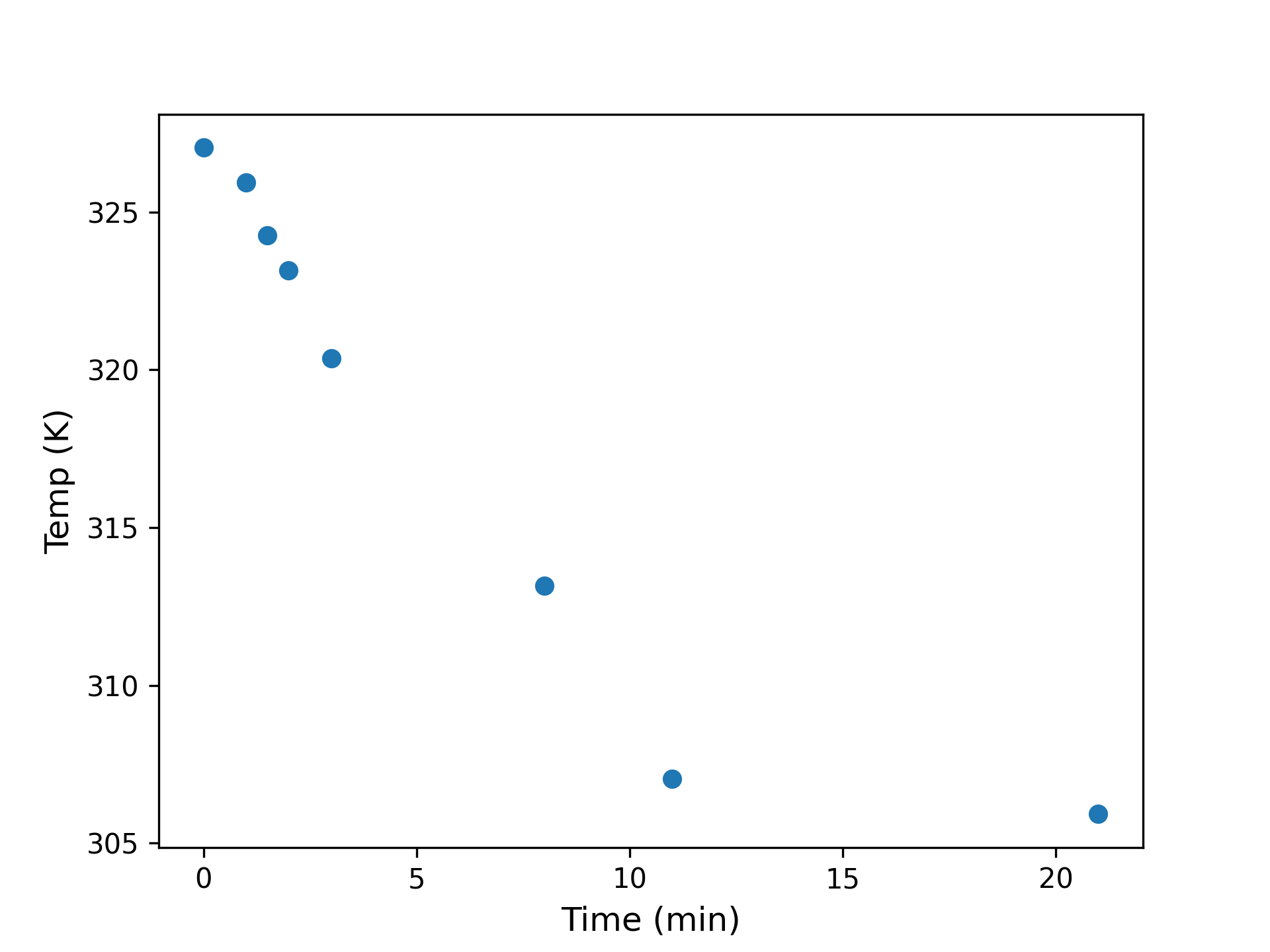
What would happen in another ten minutes? Another hour? Basic theory recommends fitting a model based on Newton’s Law of Cooling, which states:
\[\dot{T} = k (T - T_{env}),\]which is to say that the change in temperature $\dot{T}$ is proportional to the difference between the current temperature $T$ and the ambient temperature of the environment $T_{env}$. The proportionality constant $k$ governs the rate of equilibriation, absorbing details about the conductivity of the interface between object and environment, the surface area of said interface, and so on.
This equation has solutions of the form:
\[T(t) = T_0 + (T_0 - T_{env})e^{-kt}.\]To fix the initial temperature $T_0$ we can simply take the first observation, which we define to have occurred at $t=0$. To find $k$ and $T_{env}$, however, we will need to do some model fitting.
Using mean squared error as our fitting criterion, our loss function is:
\[L(k, T_{env}) = \frac{1}{N} \sum_{i=1}^N (T_i - \hat T(t_i; T_{env}, k))^2.\]While this non-linear least squares problem has no analytic solution in general, we can use a standard optimizer (in this case, the out-of-the-box Nelder-Mead solver as implemented in SciPy) in order to find the maximum likelihood parameter estimates. Our MLE parameter estimates are $\hat k \approx 0.11 (min)^{-1}$ and $\hat T_{env} \approx 302.3\mathrm{K}$. These values check out: 302K is in the eighties on the Fahrenheit scale, entirely believable for the stovetop of a recently used oven. Similarly, a cooling rate constant of $0.11 (min)^{-1}$ implies that an object heated to 350F would become touchable after fifteen minutes and completely cool within an hour. This might be slightly fast for a cake, but checks out for roasted nuts on a thin metal pan. We can therefore have some confidence that the fitting procedure has not gone completely awry.
We can also check the goodness of fit visually and confirm that our model is reasonable:
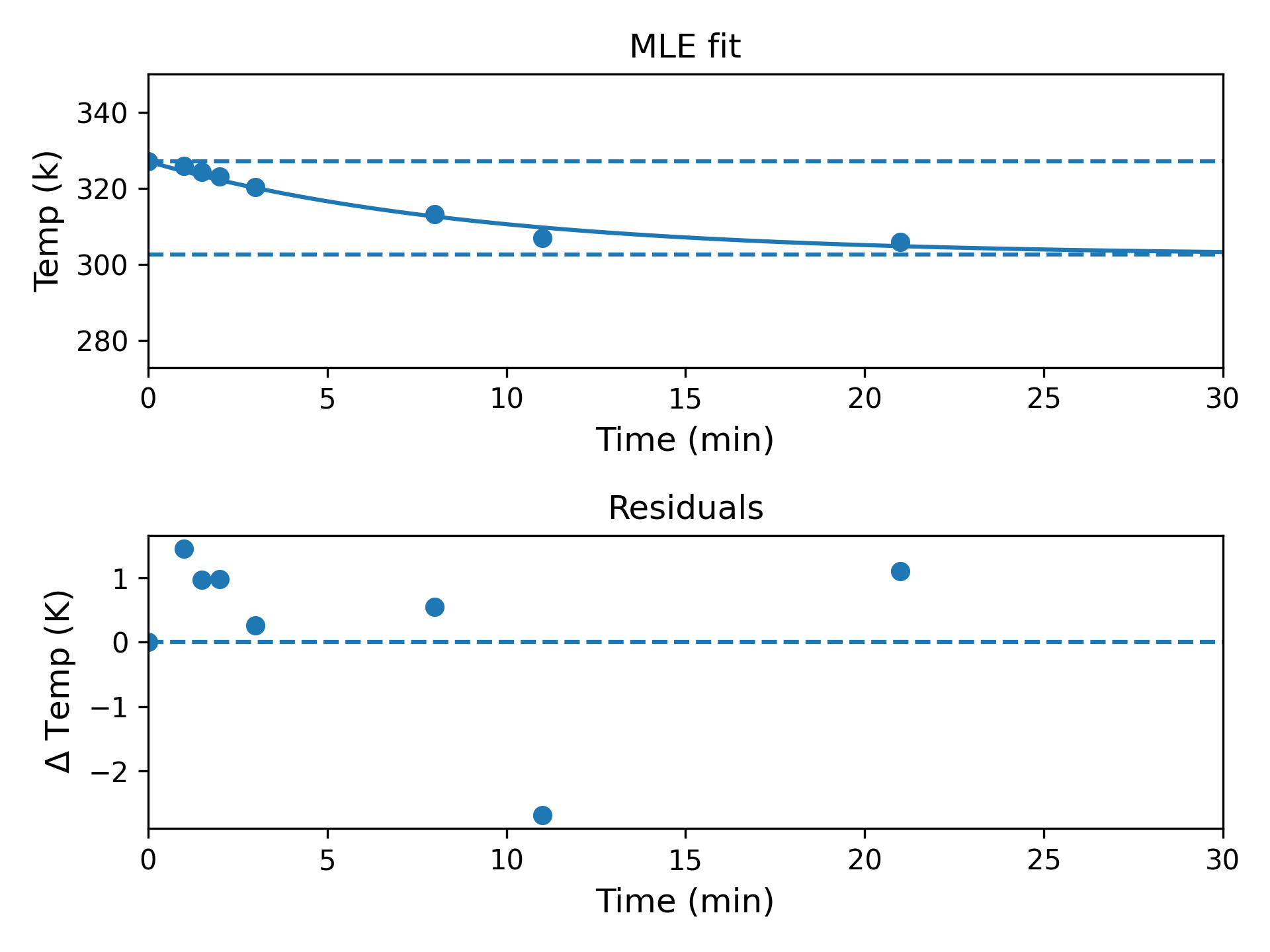
While there is some non-normality in the residuals (presumably driven by the outlying penultimate data point), this is hardly the worst model for eight observations casually collected in the kitchen with a meat thermometer and a wristwatch.
(As an aside, this should also help you to believe that this data is indeed real, because if I had faked it would have looked nicer!)
Having found reasonable point estimates for our parameters, though, we might now ask: how much uncertainty is attached to these estimates?
In order to proceed we must probabilize the model, i.e. render it in a form where it can assign probabilities to observations, given some choice of parameters. A natural choice, given that we are already fitting according to MSE loss, is to assume that our observed data is independently and identically normally distributed about the true temperature. This assumption is not merely physically plausible (if the errors are the result of many small additive sources) but is actually suggested by the loss function itself. The loss
\[L(\theta) = \frac{1}{N} \sum_i (T_i - \hat T(\theta, t_i))^2\]can be reconstrued as:
\[\ell(\theta; \sigma) = \log Z (\sigma) + \sum_i \frac{-(T_i - \hat T(\theta, t_i))^2}{2\sigma^2}\]i.e. the negative MSE is (up to a data-independent constant) just the log-likelihood of independent normally-distributed data, where the $i$th observation has mean $\hat T_i(\theta, t_i)$, and all observations share a variance $\sigma^2$. What value of $\sigma^2$ should we choose? One natural choice is to simply let the data speak for itself. We can find the value of $\sigma^2$ that maximizes its likelihood by numerically solving:
\[\sigma_{MLE} = \textrm{argmax}_\sigma \ell(\theta; \sigma).\]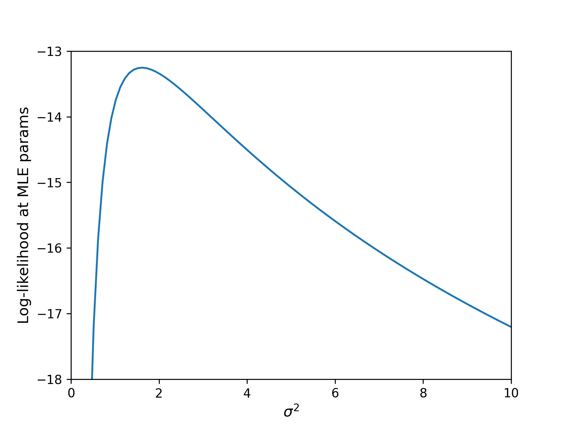
We find that the optimal noise scale is given by $\sigma \approx 1.3$K, roughly 2.3 $^\circ$F. The fact that the maximum likelihood estimate puts the typical error at about 1K (and not, say, 0.01K or 100K), is another helpful sanity check: it agrees with our intuition about the precision we can expect from a meat thermometer. In any case, 1.3 is perhaps not so different from unity as to be worth worrying about.
With the noise scale estimated, we can sample from the posterior joint distribution of $T_{env}$ and $k$ using MCMC. The resulting marginals look like this:
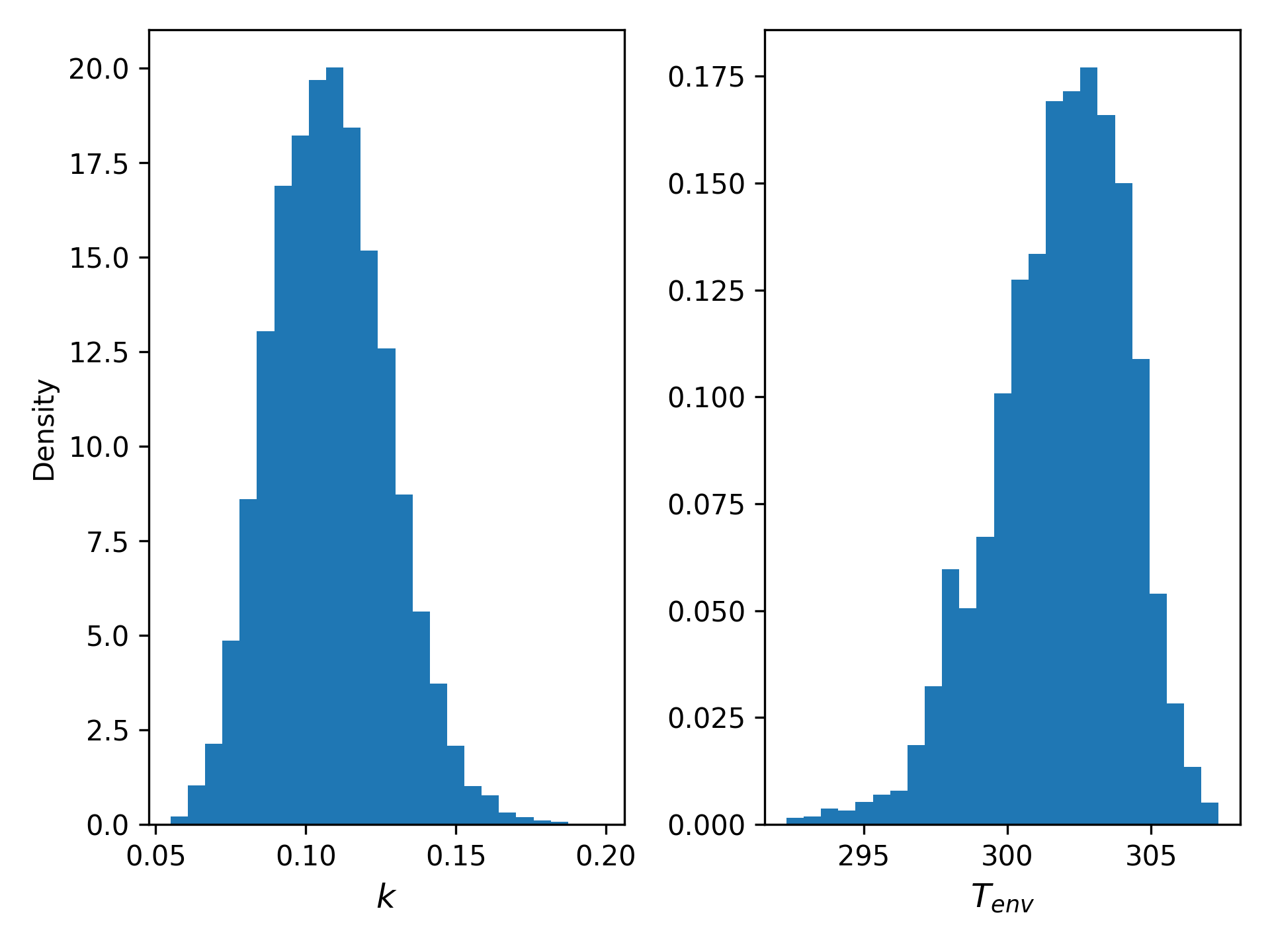
There’s a fair bit of residual uncertainty here: the standard deviation of $T_{env}$ is about 5K, and $k$ has wiggle room amounting to a factor of two in either direction.
When we examine the likelihood surface, however, a different picture emerges. In the figure below, log-likelihood is plotted as a function of $T_{env}$ and $k$. The yellow ribbon corresponds to the region of highest likelihood; the indigo basin, the lowest. MLE parameters are indicated with a red dot, and the right-most plot simply shows a zoomed-in view of the left (NB that the aspect ratios are not necessarily identical).
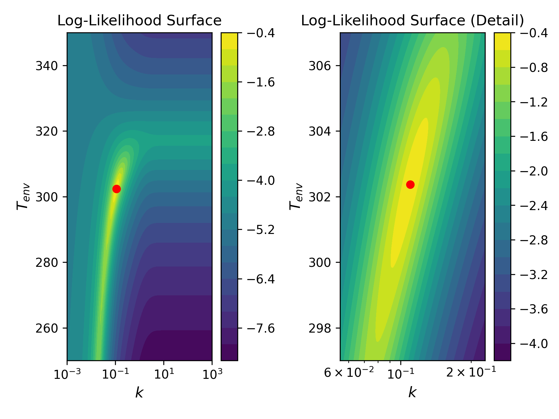
This plot bears several features that we can come to recognize as generic characteristics of physical models. For now, we can simply pick them out and list them:
- The region of high likelihood is, to a first approximation, a 1-D manifold embedded within a 2-D parameter space.
- To a second approximation, the manifold forms a kind of ribbon with one length scale many times longer than the other.
- The likelihood changes sharply in response to movement along the thin (or stiff) dimension of the manifold. Conversely, the model is practically indifferent to movement in the long (or sloppy) dimension.
- The manifold is not well-described in terms of the bare parameters of the model. Instead, taking the MLE estimate as the origin of a new coordinate frame, the stiff dimension is given by some linear combination of parameters, and the sloppy dimension by another. In words, the model is largely indifferent between cooling slowly to a lower ambient temperature or cooling quickly to a higher one. But it can tell the difference between cooling quickly to a lower temperature and slowly to a higher one.
- Because the manifold is curved (as viewed from the bare parameter space), the natural coordinate frame (i.e. directions of maximal stiffness and sloppiness) changes as a function of position along the manifold.
Conclusions (for now)
It was a pleasant surprise to find that, even in a simple two-parameter model fit with science-fair-grade data, some of the essential phenomena of model sloppiness already appear. In future posts I’d like to explore the math behind model sloppiness in more general terms and perhaps revisit our pecan cooling model through a series of increasingly powerful lenses.
References
Most of the literature on model sloppiness, as well as some introductory tutorials, can be found through Jim Sethna’s website.